All articles

Every article on this site, oldest first, as one printable page.

14 articles, 2016–2026.

My First Full-Stack Project: LEDs Driven by an FFT

A Raspberry Pi music player that drove RGB LED strips.

RGB LED strips lit by a music synchronisation project.

This was my first real project and the one that paved the way for the ATtiny85 handheld1 four years later.

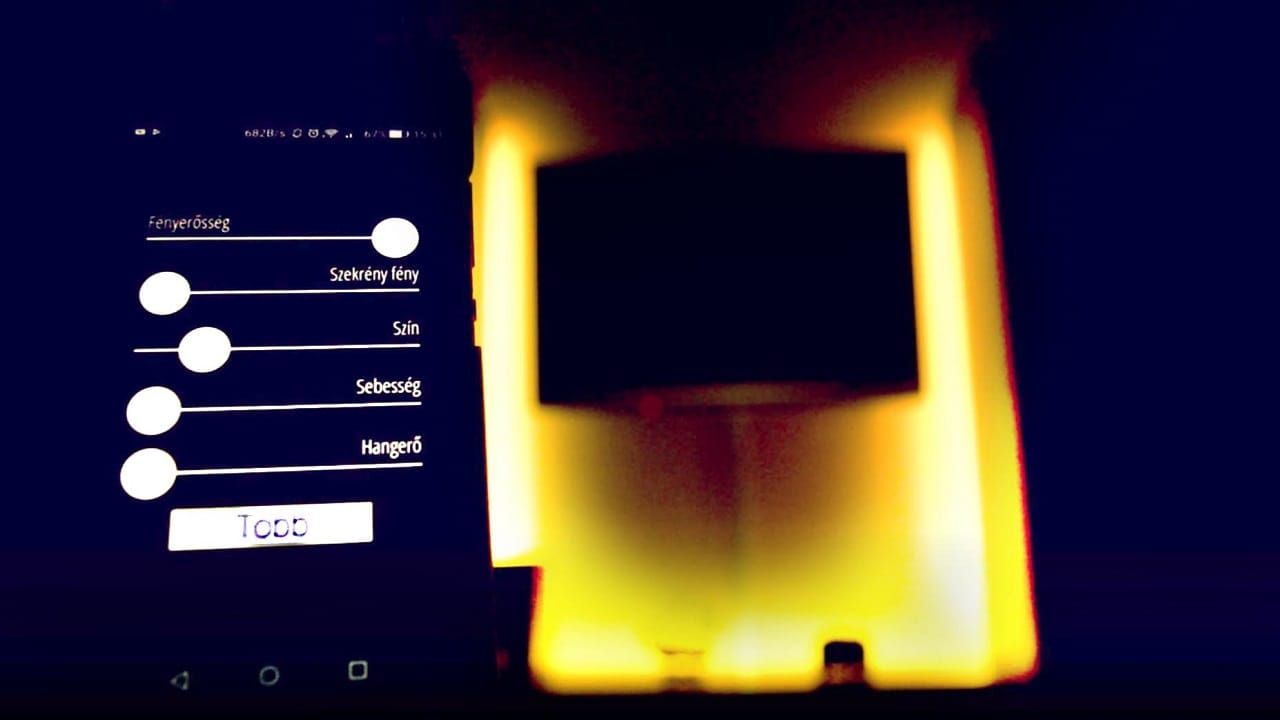
When I bought my first Raspberry Pi, a Raspberry Pi 1 Model A2, I had no idea what I was doing. Trying to drive a 12 V RGB LED strip burnt me both figuratively and literally, but it taught me how to wire MOSFETs and control them with PWM3. The obvious next step was to make the strip do something. I’d seen LEDs react to music and then stumbled across an article on the FFT4. The article was thoroughly arcane to me, but it gave me the last building block I needed.

Without quite meaning to, I’d built a full-stack application. I learnt about Ajax5 and XMLHttpRequest6, became fascinated by CSS, and discovered that programming can feel like real-life magic. I wish more kids had that first experience of programming: one that makes you curious to build things and doesn’t punish you too harshly for making mistakes along the way.

  1. ATtiny85 handheld: https://schmelczer.dev/articles/ad-astra-attiny85-game-engine/
  2. Raspberry Pi 1 Model A: https://en.wikipedia.org/wiki/Raspberry_Pi
  3. PWM: https://en.wikipedia.org/wiki/Pulse-width_modulation
  4. an article on the FFT: https://betterexplained.com/articles/an-interactive-guide-to-the-fourier-transform/
  5. Ajax: https://developer.mozilla.org/en-US/docs/Glossary/AJAX
  6. XMLHttpRequest: https://developer.mozilla.org/en-US/docs/Web/API/XMLHttpRequest

Physics Exam Practice App

How I learnt what good software actually means.

Screenshot of the Fizika practice app showing topic-selection buttons over a light textured background.

Producing value is the ultimate test of software. Users don’t care about the cool tech or clever architecture; often, they don’t even care about half the features. They have a problem they want your software to solve.

The problem

My classmates and I were preparing for the advanced physics component of the Hungarian érettségi, the secondary-school leaving exam whose results also count towards university admission. We were advised to start two years in advance by solving questions from past exams1. But the archive mixes questions from across the curriculum. That makes it tedious to practise a specific topic and hard to tell whether you’ve found a gap in your understanding or a question simply covers material you haven’t learnt yet.

The solution

I manually extracted the questions and diagrams from years of exam PDFs, a perfect way to procrastinate on studying. Then my physics teacher, the project’s other stakeholder, and I categorised every question by topic. Finally, I built a small web interface over the database. The site still runs at fizika.schmelczer.dev2, making the questions searchable and generating mock exams using only topics a student should already have mastered.

I built it early on, with only a rudimentary understanding of full-stack development. Yet it was my most popular app for years, measured by both active-user count and time spent per user. It has stood the test of time too. Students at my old school, PTE Babits Mihály Gyakorló Gimnázium3, still use it to prepare for the same exam.

The evolution of the solution

The app has gone through a few iterations. It started as the most spaghetti-like PHP app imaginable, backed by an entirely unnecessary MySQL database. But it worked. I got a good score on the exam and left the site running for future students.

Eventually, hosting a full-blown database became too expensive to justify, so I migrated everything to a static site, hosted first on Firebase, then on GitHub Pages, and now on my own server. Year after year, students emailed me asking how to add the latest questions, and guiding each of them through the GitHub workflow became tiresome. So at the beginning of 2026, I vibecoded a small CRUD interface that edits a JSON file on disk. The file is under version control, so a bad edit can always be undone. I’m back to running a backend server, but the infrastructure was already in place, so the marginal cost was negligible. Happy users, happy maintainer.

Conclusion

Two takeaways from this have shaped my values. First, data can be far more important than the app around it: Fizika’s wrapper has been replaced twice without changing its core value. Second, building software for the thrill of engineering is fun. But building software to create value at minimal cost is how you create actual value.

  1. past exams: https://www.oktatas.hu/kozneveles/erettsegi/feladatsorok
  2. https://fizika.schmelczer.dev/
  3. PTE Babits Mihály Gyakorló Gimnázium: https://babits.pte.hu/
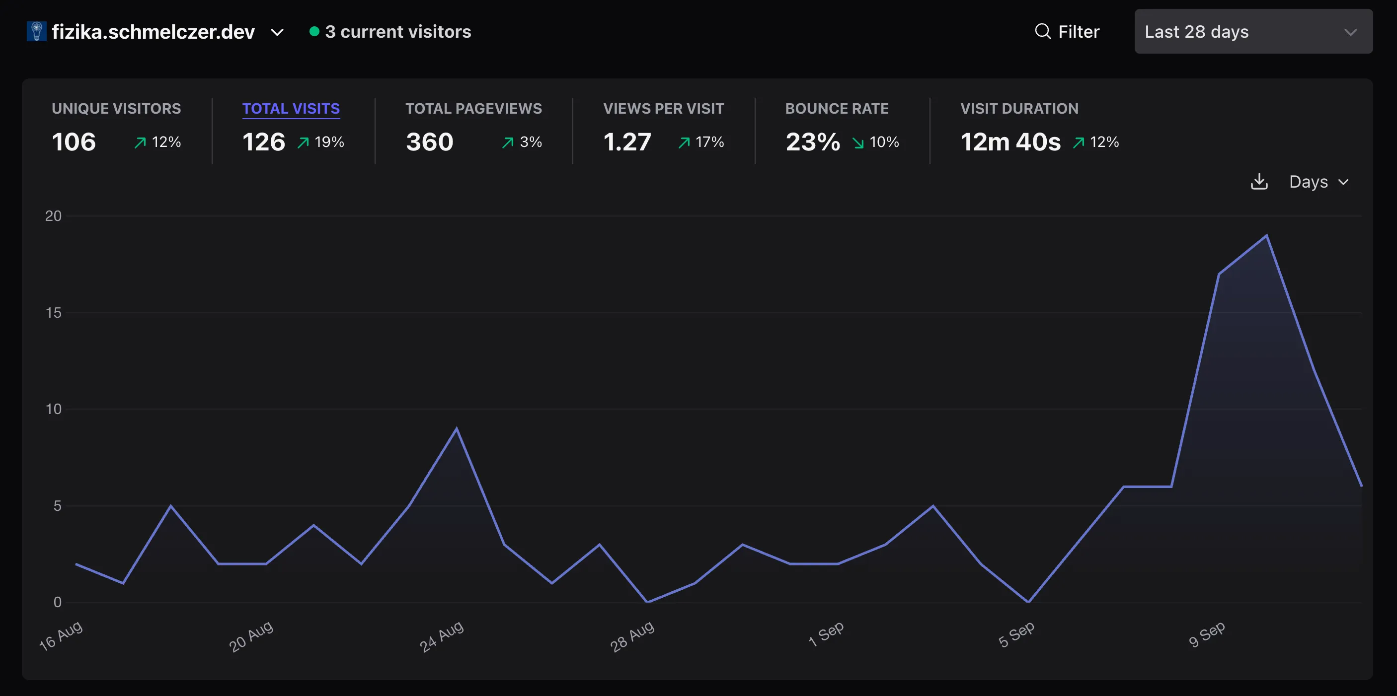
Plausible analytics dashboard showing 273 unique visitors in a 60-day window

Photo Site Generator

My photo portfolio site: once PHP on a Raspberry Pi, now a Vite script turning a folder of JPEGs into static HTML.

Screenshot of a generated photography site.

When I was fifteen, I spent the salary from my first summer job on a Nikon D32001, my first proper camera. I’ve been photographing whatever captures my imagination ever since. I wanted a personal way to share the results without using social media, which was the perfect excuse to build a portfolio site.

It started as a PHP site running on a Raspberry Pi in my room. To simplify maintenance, I replaced it with a small Vite script that takes a folder of photos and generates static HTML and several sizes of each image.

My only rule for good technology is that it must offer more value than the effort required to use and maintain it. The part of photography I enjoy is taking photos. The website itself is just a nice-to-have, so publishing must take almost no time. Committing a JPEG to a Git repository and pushing it is about the right amount of effort. It’s still one more step than the PHP version required, but I have taste in technology too, not just in photography.

  1. Nikon D3200: https://en.wikipedia.org/wiki/Nikon_D3200

My first browser game

A small game I used as the basis for SchDesign's JavaScript workshop at BME.

Screenshot of the Avoid web game.

You’re a dot; other dots come in from the edges and chase you. Your only defence is to outmanoeuvre them until they crash into each other. That’s the entire game, and it’s genuinely fun for the first few minutes: a decent return on so little code.

It was also my first time using the <canvas> element. I didn’t know it then, but that one API started an obsession with graphics programming that hasn’t let go of me since.

Later, at university, the game got a second life as the basis for our design society’s web workshop. We rebuilt it step by step with people who’d never drawn a pixel using code. It was exactly the right size: small enough to finish in a few hours, but rewarding enough to feel worth finishing. The handout offered one piece of process advice:

Get it working first, make it pretty afterwards.

That’s still roughly the only process I follow.

3D Voxel Game in C

Destructible voxel terrain, flying enemies, and a renderer derived on Post-it notes.

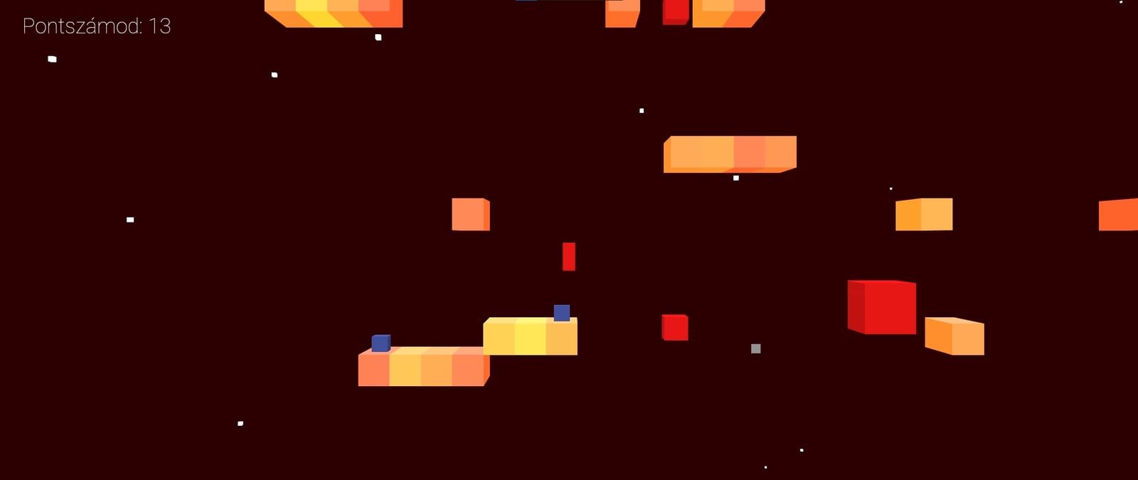
Screenshot from a 3D platform game written in C.

2026 update: I haven’t used Windows for a long time, but I’d been wanting to play this game again, and the original binary was compiled only for Windows. I’d never got around to migrating it to SDL2, but an AI agent finally let me just one-shot the migration. So the game I built nine years ago is playable again at platform-game.schmelczer.dev1.

I titled my first proper university project Platform Game. I’ve clearly come a long way since then, yet one thing hasn’t changed: I’m still bad at naming things.

Back in 2017, I created an actually fun 3D game in pure C with the help of SDL 1.22. I’d wanted to build it ever since I first downloaded GameMaker3 and realised that I could make a video game. I’d already tried with Avoid4, and Platform Game is essentially an upgraded 3D version of it.

The maps are randomly generated, but the platforms are laid out so that every jump remains possible with the player’s gravity and jump-strength settings. The world is also fully destructible, voxel by voxel. You can build structures to hide from flying enemies, although once they merge and grow large enough, they can destroy the terrain too. After collecting enough power-ups, you can shoot back or sacrifice points to slow down time.

One feature I distinctly recall is the save file format. Initially, the game dumped the entire procedurally generated map into a file, so one saved map could reach hundreds of megabytes. I realised that each map had long runs of similar voxels, mainly air at the top and ground at the bottom. Encoding those runs as repetitions massively reduced the file size. I ended up discovering run-length encoding5, although I later learnt I wasn’t the first person to do so.

One thing I didn’t discover during this project was how to do computer graphics properly: I settled on a software renderer capable only of drawing cubes after deriving a cube’s 3D-to-2D projection using trigonometry and a lot of Post-it notes. Doing it properly had to wait a few more years for a 2D ray tracer6.

I’ve made the source code public, more as a reminder to myself than as something others should learn from. The project is neither elegant nor efficient, but it produced a genuinely fun game and it made me fully realise my passion for creating virtual words.

  1. https://platform-game.schmelczer.dev/
  2. SDL 1.2: https://www.libsdl.org/
  3. GameMaker: https://gamemaker.io/
  4. Avoid: https://schmelczer.dev/articles/avoid-early-web-game/
  5. run-length encoding: https://hydrolix.io/blog/run-length-encoding
  6. a 2D ray tracer: https://schmelczer.dev/articles/sdf-2d-ray-tracing/

Explosive traffic simulation

A low-poly Unity city built for the CrySyS PLC-hacking challenge.

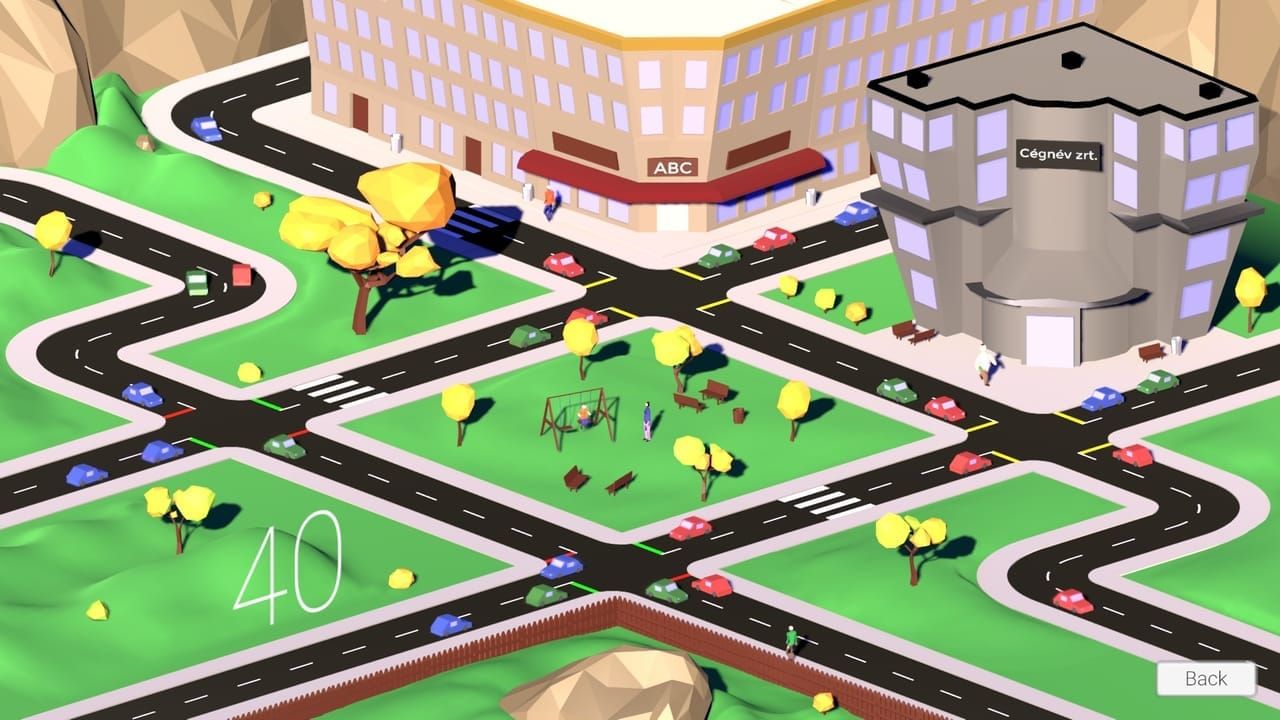
Low-poly Unity city with cars queuing at junctions around a small park.

While working at CrySyS1, the cybersecurity research group at my first university, I got the fun job of simulating traffic in a small city. The lab was preparing a hacking challenge targeting PLCs that controlled traffic lights, so a successful attack would cause mayhem on the roads.

I built everything in Unity2. C# scripts controlled the drivers, with driving and self-driving models designed to look realistic, and a REST API exposed the individual traffic lights for remote control. The drivers had to obey the lights unconditionally, tunnel vision and all. That was the point: faulty control logic had to lead to wacky disasters on screen.

The art was on me too, so I ended up watching a bunch of Blender Guru3 tutorials and modelling everything in a low-poly style. Far too much of that time went into trying to get the swing animation right; it wasn’t great, but it looked passable from a distance.

The CTF’s large venue, with screens dotted everywhere, added one final challenge: netcode. The whole simulation ran on a server, with each screen acting as a thin client that extrapolated from the latest state it had received.

  1. CrySyS: https://www.crysys.hu/
  2. Unity: https://unity.com/
  3. Blender Guru: https://www.youtube.com/@blenderguru

50 FPS Game Engine on an 8-Bit Microcontroller

A handheld game built from the PCB up: ATtiny85V, OLED, IR receiver. 8 MHz, 512 bytes of RAM, and a charming atmosphere.

The Ad Astra game running on a small OLED display.

I grew up playing with little gadgets: fake Tamagotchis, Game Boy imitations with 100+ built-in games, and the like. Naturally, I wanted to build my own.

The game

You keep a broken spaceship alive. Asteroids drift past; you mine them and spend the points on upgrades. Each upgrade unlocks either a station with a new capability or a crewmate to automate a station for you.

The hardware

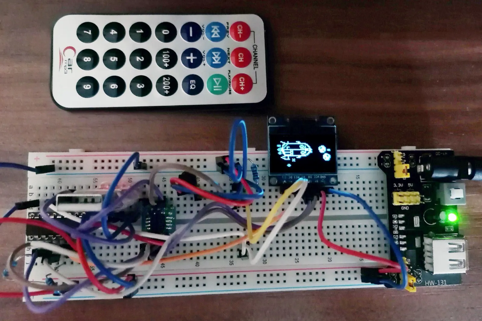
I settled on the ATtiny85V1, driving a common 128×64 1-bit OLED2. To keep the footprint small, I used an IR receiver that works with almost any remote instead of built-in buttons or a joystick. Mine was a generic hi-fi remote I bought on AliExpress for pennies. Connecting the components was quite simple, even if my breadboard suggested otherwise:

Routing the PCB from this design was relatively straightforward. The real challenge was the firmware.

Reality check

I had planned an open world, “advanced” AI, and more, but I quickly got a reality check. Even after bit-packing, the framebuffer alone would’ve needed twice the microcontroller’s 512 bytes of RAM. The 8 KB of program memory left little room for grand ambitions either. Still, I made it work.

Rendering engine

To achieve 50 FPS and fit into RAM, the engine renders at a quarter of the display’s resolution (64 by 32 pixels). The OLED’s zoom setting doubles the image vertically, while sending each byte twice over the wire doubles it horizontally. This gives nearest-neighbour upscaling without storing any extra pixels.

The screen’s pixels are either on or off, so 1 bit per pixel should be enough. But a rendering engine also needs compositing, which requires a second bit per pixel to represent transparency. That’s what lets the black pixels inside the spaceship’s sprite hide the stars behind them, while the black pixels outside it stay transparent and let the stars show through.

A shortcoming of this scheme is that it uses 2 bits per pixel for only three distinct states: black, white, and transparent black. Transparent and opaque white both produce a white pixel regardless of what’s behind it.

After realising this, keeping the entire framebuffer in memory seems impossible once again: 64 × 32 × 2 bits is exactly the amount of RAM the microcontroller has, leaving nothing for the game itself. The pragmatic choice would’ve been a bigger microcontroller, but hobby projects don’t always have to be pragmatic. I carried on and made the renderer stream 8 bits at a time, resulting in 32 render passes per frame. Each pass processes 8 pixels in parallel in a SIMD-like fashion.

Sprites are stored as 16-bit columns (matching the word size of the EEPROM): the high byte is a mask, and the low byte contains the fill bits. Compositing eight vertical pixels of a sprite onto the framebuffer is a single expression:

newColumn = oldColumn & transparencyMask | fill;

The sprites are C arrays injected into the source code by a Python script, so the somewhat strange layout doesn’t leak into the sprite creation workflow.

Game logic

For the game engine’s scripting model, I borrowed ideas from JavaScript prototypes3 and Unity objects4. Of course, the size constraints allowed only a lightweight version. All game objects live in one array. Each object holds a union of possible object states and a pointer to its actual prototype: essentially a virtual function table5 containing the object’s tick (to update the object and interact with others on every game tick) and draw functions. Although simulation and rendering share the same 50 Hz tick, they need separate functions because draw renders one 8-pixel stripe at a time and may run several times per object per frame. This quasi-vtable doesn’t become a bottleneck either. The beauty of the ATtiny is that it only has SRAM, with no complex prefetching or line faults to make jumping around in memory expensive.

In the end, the game does have “AI” too, in the form of a finite state machine. Your astronaut crewmates have a prioritised list of activities to attempt based on the player’s current activity.

Saves

The game’s binary already fills the 8 KB of program memory, so the sprites have to live in EEPROM. There is still enough room alongside them for a save file: a few dozen bytes containing the serialised game-object list. To prevent an unexpected shutdown from corrupting the save, the EEPROM holds two save buffers and a flag identifying the last completed one. The flag flips only after the older buffer has been fully overwritten, making saves atomic. It all happens in the background through interrupts to avoid jitter in the rendering loop.

Was it worth it?

Absolutely. Don’t get me wrong, the gameplay gets old after 15 minutes. You spend the first five completing the game, then watch your crewmates run the spaceship as a soothing loop emerges from their state machines.

Reading the datasheets cover to cover, understanding the limits, and learning how to push them was incredibly fun. This is about as full-stack as a project gets, and it made me think about performance on a completely different scale from what I was used to.

By the end, though, the game and my software-UART logging code no longer fit in program memory at the same time, so I had to disable parts of the game whenever I needed logs. If I built it again, I’d start with a simulator. Skipping the flashing step would speed up iteration and make “there’s no output, what now?” failures much easier to debug. It would also enable end-to-end tests in CI. An 8 KB program can only hold so much complexity, but developing anything larger without better testing would’ve been prohibitively slow.

  1. ATtiny85V: https://ww1.microchip.com/downloads/en/DeviceDoc/Atmel-2586-AVR-8-bit-Microcontroller-ATtiny25-ATtiny45-ATtiny85_Datasheet.pdf
  2. 128×64 1-bit OLED: https://www.olimex.com/Products/Modules/LCD/MOD-OLED-128x64/resources/SSD1306.pdf
  3. JavaScript prototypes: https://developer.mozilla.org/en-US/docs/Web/JavaScript/Inheritance_and_the_prototype_chain
  4. Unity objects: https://docs.unity3d.com/Manual/Components.html
  5. virtual function table: https://eli.thegreenplace.net/2013/12/05/the-cost-of-dynamic-virtual-calls-vs-static-crtp-dispatch-in-c
A breadboard threaded with jumper wires, carrying the ATtiny85, an IR receiver, a power module, and the OLED mid-game, with a small remote beside it

One Game Library, Imported by Both the Client and the Server

A mobile multiplayer browser game where client and server linked the same TypeScript module. One source of truth, one fewer class of bug.

The decla.red browser game interface showing a space scene.

2026 update: I recently revived the game: modernised the toolchain, made it more fun, rebranded it as doppler, and rewrote the netcode. It’s playable at doppler.schmelczer.dev1. The section near the end covers what changed; everything before it describes the 2020 original.

My BSc thesis was a renderer; decla.red was the proof that it could survive contact with a real game. In autumn 2020, I built a conquest-style space shooter on top of SDF-2D2: two teams fight over tiny planets with actual gravity, everything is ray-traced, and it all runs in a phone’s browser. The teams are called decla and red, which is how the game got its domain. The decision I still think about, though, came from a less glamorous need: stopping the client and server from disagreeing about what the game even was.

One package, both sides of the wire

Real-time multiplayer hands you an awkward two-machine problem. The server has to be authoritative or the game is cheatable; the client has to feel immediate or the game is unplayable. Write the rules twice, once per side, and they drift: slowly at first, then visibly, with a player’s screen saying one thing while the server believes another.

So the whole object model lives in a single shared package that both sides’ package.json files pull in with file:../shared. Every entity exists in three layers. A PlanetBase in the shared package holds the data format and the rules both sides must agree on. The server subclasses it into a PlanetPhysical, adding the collision outline, gravity, and ownership; the client subclasses it into a PlanetView, adding the drawable and the ownership ring. Characters, projectiles, and lamps follow the same pattern. The server simulates at 200 Hz, each of its instances hosting 16 players by default, with bots filling the seats humans haven’t taken, and sends every client a snapshot 25 times a second.

The class name is the protocol

The snapshots go through a serialiser that is ten lines long, and I’m still fond of it:

export const serialize = (object: any): string => {
  return JSON.stringify(object, (_, value) => {
    if (value && value[mangledTypeKey]) {
      const props = value.toArray() as Array<any>;
      props.unshift(value[mangledTypeKey]);
      return props;
    }
    return value?.toFixed ? Number(value.toFixed(3)) : value;
  });
};

An object crosses the socket as [className, ...fields], with every number rounded to three decimal places on the way out. Deserialisation is the mirror image: a JSON.parse reviver looks up the first element in a registry and calls the matching constructor with the rest. And since JSON.parse revives from the inside out, nested objects are already live instances by the time the outer constructor runs.

The registry is what lets the three class layers cooperate, and decorators wire it up:

// on the server
@serializesTo(PlanetBase)
export class PlanetPhysical extends PlanetBase { ... }

// on the client
overrideDeserialization(PlanetBase, PlanetView);

A PlanetPhysical leaves the server labelled PlanetBase and materialises on the client as a PlanetView. Neither program ever learns the other’s class names; the only contract is the base class’s constructor signature.

Keying a protocol on class names has one famous enemy: the minifier. The frontend and the backend are two separately minified bundles, so PlanetBase gets mangled into two different single letters, the registry lookup fails, and every packet quietly deserialises into a plain array. The fix took two commits in October 2020: the first switched the minifier off altogether, and the next day’s commit3 turned it back on with a webpack option telling it never to rename classes. It taught me early that “works in dev, breaks in prod” usually means a build tool was being clever somewhere out of sight.

messageNotUnderstood

Messages in both directions of the protocol, and most calls inside each program, use batches of Command objects. A command’s type is its class name (the minifier constraint, again), and every actor extends a CommandReceiver: a lookup table from command type to handler, plus a defaultCommandExecutor for everything else. I borrowed the idea from Smalltalk4’s message passing, doesNotUnderstand: included.

The default handler is where it gets fun. Containers default to broadcasting: the server’s physics container forwards any command it doesn’t recognise to every object it holds, so one StepCommand advances the whole world. The client’s socket wrapper defaults to queueing the command for the server. Nothing on the client handles a MoveActionCommand, so when the keyboard listener emits one, it falls through the default handlers and lands on the wire, addressed to the one machine that does understand it. Extending the game meant adding a command and a handler, not reorganising an inheritance tree.

Sphere tracing on the server

SDF-2D never sees a triangle: every shape is a signed distance function. The server has no pixels, but it kept the fields. A moving circle is checked for collisions using sphere tracing, the same algorithm the renderer uses to march light rays: advance by the field’s value, which is by definition a safe step, until the distance is covered or the field dips below the circle’s radius. On a hit, the surface normal comes from sampling the field 0.01 units on either side of the hit along each axis, and both parties receive a ReactToCollisionCommand: the projectile learns it should bounce, the character learns it should bleed. Rendering, lighting, and collision speak the same geometric language, so each shape in the game is defined exactly once.

The shapes themselves are modest: planets are seven-sided polygons with jittered vertices, and characters are three circles, a head and two feet, which the character shader melts into a single creature. Gravity is defined per planet and tuned by hand rather than physically accurate: the pull is 5000 * ((800 / d) ** 1.5 - 1), clamped to 50,000, where d is the distance beyond the planet’s mean radius. It’s exactly zero beyond 800 units, so most of space stays calm, and it saturates up close, so orbiting near a surface feels sticky instead of chaotic.

A k-d tree with four dimensions

Once the world held more than a few dozen objects, the question “what’s near this circle?” dominated the server tick. Static objects therefore live in a k-d tree5 with a trick I remain pleased with: each axis-aligned bounding box is treated as a point in four-dimensional space (its two x-bounds and two y-bounds), and the tree cycles through those four coordinates level by level, discarding provably non-overlapping subtrees along the way. Dynamic objects, the dozens of characters and projectiles, stay in a plain array that gets filtered linearly; at that count, a tree would cost more to maintain than it saves. The static tree is built once at world generation and never rebalanced, which is fine, because planets don’t move.

Bandwidth on a diet

Each player only hears about objects near their view. The view box starts with a constant area budget, four 1080p screens’ worth of world, takes its shape from the client’s reported aspect ratio, and is then enlarged by 20%. A portrait phone and an ultrawide monitor see the same amount of world in different shapes. Every 40 ms, the server diffs the box’s contents against the previous cycle. Newcomers arrive as fully serialised objects, leavers as a list of IDs to delete. Players beyond a slightly smaller box get special treatment: the client receives only a normalised direction vector for each, enough to draw an arrow at the edge of the screen, not enough to reveal where anyone actually is.

Within the box, every property update carries not just a value but also its rate of change. Between snapshots, the client advances each property along its streamed derivative, and when the next snapshot disagrees with the guess, the error is not corrected with a jump: it’s folded in as an extra velocity spread over the following 33 ms, bending the object back onto the true path. Only a discrepancy of more than 200 units, such as a respawn or a teleport, causes an immediate snap. In 2020, this was the whole story. Your own character was extrapolated like everything else, so every input took a round trip before it moved you. The shared package made real prediction possible; cashing that cheque took another six years.

Other choices worth a sentence

  • Bots with 1 Hz brains. NPCs re-plan once a second, consider shooting twice a second with a coin flip and up to 200 units of deliberate aim error, and re-roll their wanderlust every three seconds. A bot that strays outside the world turns back and doesn’t resume hunting until it’s well inside again, so it never dithers at the boundary. The roster of 48 names includes Sisyphus, who keeps trying.
  • Reinforcements, not respawns. A player’s new character spawns next to a living teammate when one exists (bots take their chances at a random spot), which quietly turns every respawn into help arriving.
  • A slow-motion ending. When a team reaches the score limit, the server divides the timestep by an exponentially growing factor, so simulated time halves every real second and the final shots sail through space in slow motion. Then it regenerates the world and everyone rejoins.
  • Server discovery via Firebase Remote Config. The list of live servers was a JSON string in Firebase Remote Config6, so adding a server required only an edit in a web console, with no redeploy. The join screen fetched the list, then asked each origin’s /state endpoint for its name and player count, retrying every eight seconds and silently dropping any that didn’t answer; once a server was listed, its live count arrived over the socket. Today it’s a hardcoded list, which is what it should have been from the start.

The 2026 revival

Six years later, I dusted the game off, and the branch (“Modernise & make fun”, says the merge commit) became a study in how my approach to writing multiplayer code had changed.

The extrapolators are gone. The character-movement code moved from the server into the shared package, so the client now runs the same stepCharacterMovement function as the server. Every input is stamped with an integer millisecond timestamp (integers survive the serialiser’s rounding; there’s a test for that now). The server acknowledges how much of your input each snapshot reflects, and the client replays the unacknowledged remainder on top of the authoritative pose, at the same 200 Hz as the server. Corrections ease in over 60 ms; a discrepancy beyond 250 units is treated as a respawn or teleport rather than a prediction error and corrected immediately. Other entities are rendered 100 ms in the past, interpolating between buffered snapshots and coasting on the streamed rates of change only when the buffer runs dry.

Sharing the simulation raised a requirement 2020-me never faced: determinism. Floating-point addition isn’t associative, so the character’s centre is computed as ((head + leftFoot) + rightFoot) / 3 on both sides, with a comment forbidding reassociation, and a test steps the shared simulation through 300 ticks of scripted input and compares the result against a pinned reference pose. The serialiser got its tests first, on the grounds that it’s the mechanism with the highest blast radius. And remote method calls sent over the wire now pass through an allowlist, because dispatching function calls using raw strings from the network is the kind of idea 2020-me found elegant and 2026-me finds alarming.

What I’d change

  • Observability for desync. Multiplayer systems live or die by visibility into divergence. I had logs; I needed to see the rate, the shape, and the triggering interaction for every extrapolation miss. Without that, debugging was guessing.
  • Untangle rendering from networking. Both were interesting, both pushed on the architecture in different directions, and their directories slowly grew into each other. Give them separate top-level homes from day one next time.
  • Skip multi-server until the maths demands it. I wrote Helm charts in the project’s first week because it sounded like the serious thing to do. There wasn’t even a game server yet, and the one that arrived three months later held 16 players; I was nowhere near needing them, and the complexity wasn’t free.
  1. https://doppler.schmelczer.dev/
  2. SDF-2D: https://schmelczer.dev/articles/sdf-2d-ray-tracing/
  3. the next day’s commit: https://home.schmelczer.dev/git/andras/decla-red/commit/d34f25295c2b73c28fc44e9223ef00b8c78d508e
  4. Smalltalk: https://en.wikipedia.org/wiki/Smalltalk
  5. k-d tree: https://en.wikipedia.org/wiki/K-d_tree
  6. Firebase Remote Config: https://firebase.google.com/docs/remote-config

A Real-Time 2D Ray Tracer That Runs on Phones

A TypeScript 2D ray-tracing library using signed distance fields. Tiled rendering and generated shaders enable real-time graphics on phones.

SDF-2D browser demo with soft lighting effects.

My BSc thesis needed two things: a renderer and something to render. The renderer became SDF-2D, a browser-based 2D ray tracer built on signed distance fields. The other half became decla.red1, a multiplayer space shooter built on it. This article is about the renderer.

2D games mostly composite unlit sprites while running on ever-faster GPUs. Ray tracing would give them shadows and area lights, and in 2D it is nearly cheap enough for a phone. Most of the thesis is about closing that gap.

Circle tracing

Sphere tracing (Hart, 1996) renders surfaces defined by a signed distance field (SDF) by marching along each ray in steps equal to the field’s value at the current point. Circle tracing is the 2D version. The geometry itself needs no rays: a negative field value means the pixel is inside an object, and values near zero give antialiasing. Rays are only needed for lighting, so performance depends on how often the field is evaluated.

Here’s a minimal scene in TypeScript, with a circle orbiting a light:

import { CircleFactory, CircleLight, hsl, runAnimation } from 'sdf-2d';

const canvas = document.querySelector('canvas');
const Circle = CircleFactory(hsl(180, 100, 40));

const draw = (renderer, time) => {
  renderer.addDrawable(
    new Circle([150 + 50 * Math.cos(time / 1000), 75 + 50 * Math.sin(time / 1000)], 25)
  );
  renderer.addDrawable(new CircleLight([150, 75], hsl(270, 100, 40), 0.1));
  return true; // flag that more frames are coming
};

runAnimation(canvas, [Circle.descriptor, CircleLight.descriptor], draw);

The descriptor list at the end looks redundant, but the shader generator needs it; more on that below.

Two passes and a grid

The naive renderer evaluates the field pixels × lights × steps times per frame. Deferred shading cuts this to once per pixel: one pass renders the distance field and base colour into a texture, and the lighting pass reads it back. The distance texture defaults to half the canvas’s resolution, and nothing visibly changes.

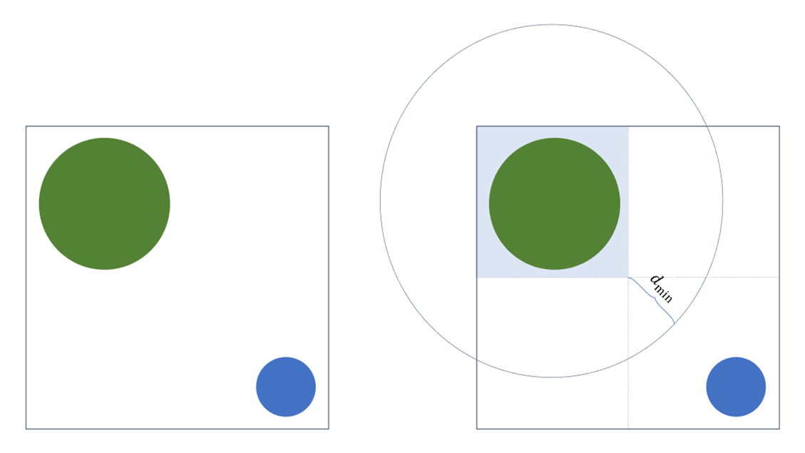
The second fix borrows from tiled renderers. The screen is split into an 8 × 8 grid, and each tile receives only the objects whose CPU-side lower-bound distance puts them within reach; its field is capped at the distance of the nearest object left out. In my 200-object test scene, the average tile needed only 23 objects.

Here are the results for that scene (200 objects, two lights, 16 shadow steps, 2560 × 1080, a desktop RX 590), with GPU time measured using EXT_disjoint_timer_query:

Optimisations enabledFPSGPU draw time
None7.5130 ms
Memoised distance field60 (capped)5 ms
Memoised field and tiles60 (capped)1.85 ms

That’s a 70-fold speed-up, giving a mid-range phone enough headroom.

Shadows in 16 steps

The textbook route to soft SDF shadows is Quilez’s ray-marched penumbra technique2. My implementation needed 64 to 128 steps per light and an exact field rather than a lower bound, yet still showed artefacts at sharp edges. I replaced it with a heuristic: march towards the light for 16 steps, divide the distance travelled by the distance to the light, and raise the ratio to the power of 0.3.

float shadowTransparency(float lightDistance, vec2 lightDirection) {
  float rayLength = 0.0;

  for (int j = 0; j < 16; j++) {
    rayLength += max(0.0, getDistance(uvCoordinates + lightDirection * rayLength));
  }

  return min(1.0, pow(rayLength / lightDistance, 0.3));
}

The closer the ray gets to the light, the less shadow its starting point receives. The heuristic has no physical basis, but it runs several times faster and accepts lower-bound fields. Anything from 8 to 32 steps looks acceptable. Light attenuates as 1 / (d / intensity + 1)² and penetrates objects at reduced intensity. One known bug: an object already inside another’s shadow darkens that shadow again, though rarely noticeably.

Shaders written by a program

WebGL1 requires loop bounds to be compile-time constants, and WebGL2 unrolls fixed-bound loops. A library can’t know how many circles you’ll draw, so SDF-2D generates its shaders at runtime. Each drawable’s descriptor declares its GLSL distance function, the uniform arrays carrying its instances, and the object counts to compile for, such as [0, 1, 2, 4, 8, 16]. The generator substitutes these into GLSL templates and compiles a program for every combination across drawable types; the count grows exponentially, but keeping it under a few hundred wasn’t hard. Each tile is drawn with the smallest program covering its object counts. Compiling them all before the first frame is why the library relies on KHR_parallel_shader_compile where available: JavaScript is single-threaded, but the driver compiling shaders is not. It’s also why runAnimation needs the descriptors up front: every drawable type must be known before the shaders are written.

Surviving the browser

The library supports WebGL1 alongside WebGL2 because, in 2020, iPhones left no choice. Both are wrapped in one context type carrying an isWebGL2 flag, so the shared path type-checks and every WebGL2-only feature has a fallback: float render targets degrade to 8-bit, parallel compilation to synchronous, the timer query to nothing. Context loss is handled too. A JavaScript Proxy around the context throws on every call once the context-lost event fires, unwinding the frame; a proxy around the renderer catches that, caches settings changed meanwhile, and rebuilds the renderer on restore. A simulator that lost and restored the context at random intervals shook out the bugs.

Field testing in an electronics store

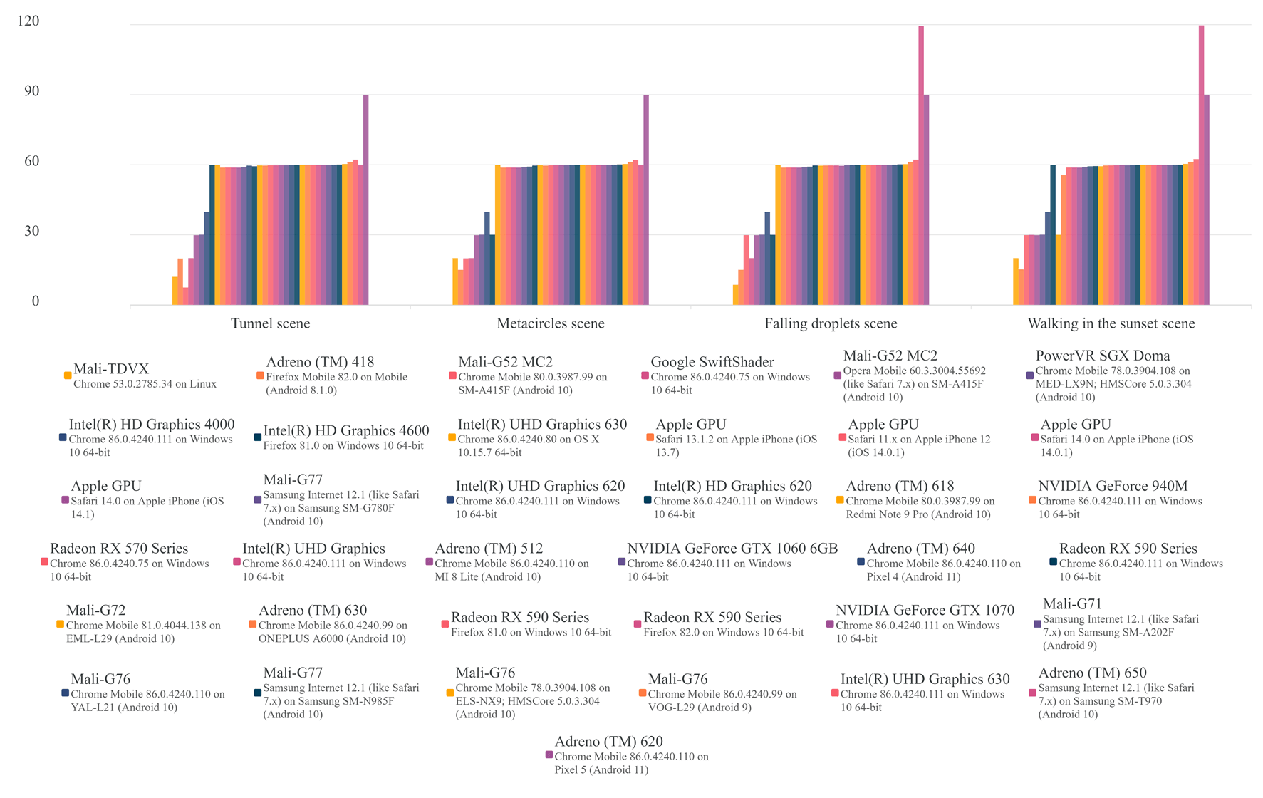
The demo page3 anonymously logs each scene’s frame rate and the autoscaler’s resolution scales. Organic visitors and pestered acquaintances provided some data; I gathered the rest by running the demo on every device on display in an electronics store, since device farms charged more than a student could afford. Of 37 unique devices, 33 held 30 FPS or better, and over three quarters stayed at the browser’s 60 FPS cap in every scene. The bars above 60 represent a 120 Hz Samsung tablet and a 90 Hz Pixel 5; the slowest results include the SwiftShader software renderer and a 4K TV running a four-year-old version of Chrome.

The data fed back into the autoscaler, which trades resolution for frame rate: I lowered its target from 50 to 30 FPS and added motion blur so weaker devices still felt smooth. Years later, Fleeting Garden4 took the same approach, shedding agents instead of pixels.

Limitations

  • Objects reach the GPU as uniform arrays, whose capacity is capped by the GPU, driver, and browser, so a complex enough scene hits a wall. The planned fix was a non-uniform tile grid, finer where the scene is busy.
  • There are two light types, a circular area light and a torch-like directional one, and no custom lighting models.
  • The banding around lights bothers me to this day. Dithering would hide it but seemed too expensive at the time.

The library is still on npm and gets a few dozen downloads a week; I like to imagine somebody, somewhere, is using it. The demo scenes are still live.

  1. decla.red: https://schmelczer.dev/articles/declared-shared-simulation-code/
  2. Quilez’s ray-marched penumbra technique: https://iquilezles.org/articles/rmshadows/
  3. demo page: https://sdf2d.schmelczer.dev/
  4. Fleeting Garden: https://schmelczer.dev/articles/fleeting-garden-webgpu-drawing/
The same sunset scene rendered twice, with the distance field at full resolution on the left and at a third of the resolution, linearly interpolated, on the right, with no visible difference
Diagram of a screen split into four tiles, where the top-left tile only needs to evaluate the green circle inside it and a larger circle marks the distance beyond which its field is no longer trusted
The same scene shadowed with 32, 16, and 8 ray steps from left to right, the shadow&#x27;s edge getting softer with fewer steps
Bar chart of frames per second for 37 device and browser combinations across four demo scenes, with most bars at 60, a few phones and integrated GPUs between 10 and 40, and two high-refresh-rate outliers at 90 and 120
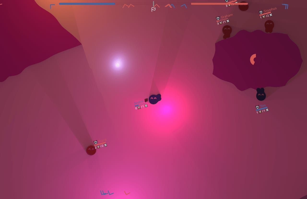
Four portrait phone screenshots of the demo scenes: blue and pink light beams between dark blobs, a magenta field of falling droplets, a purple ridge lit from two sides, and a red figure on a hill at sunset

Keep It Stupid Simple Backup Strategy

A shell script so simple I'm willing to trust it with my most precious data.

The BorgBackup logo, with the word Borg in green stencil letters on a black background.

The more critical a system is, the simpler it should be. In practice, that means building on battle-tested foundations and adding only the thin layer of logic that’s strictly necessary.

My home server’s backup is a good example. I aim to use SQLite wherever I can, but my self-hosted stack has grown to include several Postgres instances, Redis, message queues, and more. This couldn’t stop me from wanting Time Machine-style backups with granular file history, which means backing up often: hourly, in my case. Shutting down the stack every hour would’ve greatly inconvenienced its active user base of two, my partner and me, so I chose to back up everything live.

I could have gone down the rabbit hole of coordinating dedicated backup tooling: a bespoke method for every service, each with its own failure modes. That would have been anything but simple. Instead, I rely on the databases’ battle-tested crash-recovery paths.

With that assumption, the backup container needs just a simple shell script. All container volumes live in the same Btrfs1 subvolume, so the script can take an atomic snapshot of all state. It then feeds the snapshots into Borg2, which provides incremental, deduplicated storage for local and SSH backup targets. A database restored from one of these backups is in a state indistinguishable from that left by a power cut. The backup script supplies only the plumbing: configuring Btrfs and Borg, handling failures gracefully, and exposing a health-check status when human intervention is needed.

I’ve been using this since 2023. I’ve restored various files and folders and performed two full (albeit planned) disaster recoveries. Nothing builds confidence like a restore that works: Borg, Btrfs, and this little script have worked well, and I don’t expect to migrate away any time soon.

  1. Btrfs: https://btrfs.readthedocs.io/en/latest/
  2. Borg: https://www.borgbackup.org/

A Fleeting Garden on Your GPU

A WebGPU physarum simulation where you can control millions of agents with your paintbrush and watch them bring your drawings to life.

Magenta, violet, and yellow agent trails looping into a mirrored, kaleidoscopic mesh on a near-black canvas.

Watching art emerge from millions of independent agents is fascinating for a while, but not for all that long. My favourite art makes the viewer part of the work, so this project had to be interactive to live up to my expectations. I was inspired by Sebastian Lague’s slime mould video1 and Sage Jenson’s work2, but I wanted more control over a running simulation rather than just passively observing it.

Architecture

A few compute shaders manage the agents’ lifecycle by updating an array in place. Each agent follows a simple loop. On every iteration, it takes three samples: one ahead and one on either side. It then goes straight, turns left, or turns right based on which sensor reports the strongest trail scent left behind by other agents. The samples come from a trail map that records the agents’ paths and slowly diffuses them over time. Its R, G, and B texture channels each hold deposits from one agent type. I considered using the fourth channel too, but three colours already make the result busy enough, and a fourth would’ve made colour theory a fair bit harder for my colour-blind eyes.

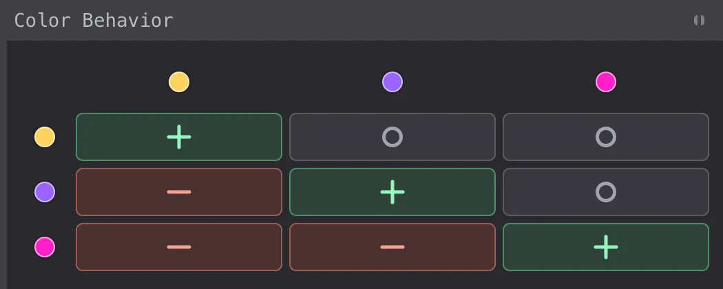
The website has multiple scenes, each with its own simulation parameters. Each scene also has a matrix that defines how every agent type responds to every other type’s trail: with attraction, repulsion, or indifference.

Make it good

My first experiment let the user draw over the trail texture, nudging the mould to change direction. That proved one layer too indirect: it barely changed the agents’ behaviour unless the effect was strong enough to make the strokes look overly thick. In the final version, drawing spawns new agents along the pen’s path. When there are too many agents on the canvas, old ones get removed as new ones arrive.

Drawing is great fun, but not everyone can draw well. No amount of line smoothing will change that, though it helped me a little. That’s why I added mirroring, a common drawing-tool feature that turns scribbles into artsy kaleidoscopic patterns.

To deepen the immersion and give each stroke more weight, I added procedurally generated piano sounds that reward drawing with increasingly complex note progressions.

I’m a firm believer that small touches give experiences polish. For instance, the toolbar samples a 13×7 grid of pixels behind it and adjusts its opacity to stay legible against any background. And the first thing a visitor sees is 180,000 agents drawing the word Fleeting with their trails, then wandering off as the simulation takes over and the letters fall apart.

Then make it fast

The simulation is split into six conditional compute-and-render stages across ten WGSL files: agent step, diffusion and decay, brush, eraser (one variant clears trails, the other removes agents), agent generation with resizing and compaction, and the final palette render.

The first step in making shaders fast is to keep the logic simple and mostly branch-free. A few other ideas helped too:

  • Agents write deposits directly to a storage texture without blending, which concurrent compute writes don’t support anyway. If two agents hit the same pixel, one deposit may be lost, but the next diffusion pass spreads the surviving deposit across neighbouring pixels, so we don’t need to sacrifice parallelism.
  • Keeping the agents packed together in memory took more care. During compaction, each workgroup uses a prefix sum to find positions for its surviving agents, so compaction needs just one atomic operation per workgroup instead of one per agent.
  • The agent count also adjusts to the frame rate. It starts at a million and drops by 200,000 per second when the smoothed rate falls below 54 FPS (90% of the 60 FPS target), down to a minimum of 50,000. A weaker device gets a thinner garden instead of a slideshow.

Give it a try

A blog post can only do so much to describe an immersive artwork. The best way to understand it is to try it, preferably with the sound on: fleeting.schmelczer.dev3.

  1. Sebastian Lague’s slime mould video: https://www.youtube.com/watch?v=X-iSQQgOd1A
  2. Sage Jenson’s work: https://cargocollective.com/sagejenson/physarum
  3. https://fleeting.schmelczer.dev/
Three-by-three matrix showing the interactions between three trail types

Compounding Self-Hosting

Combining Immich, Home Assistant, and an e-ink screen for truly personal tech.

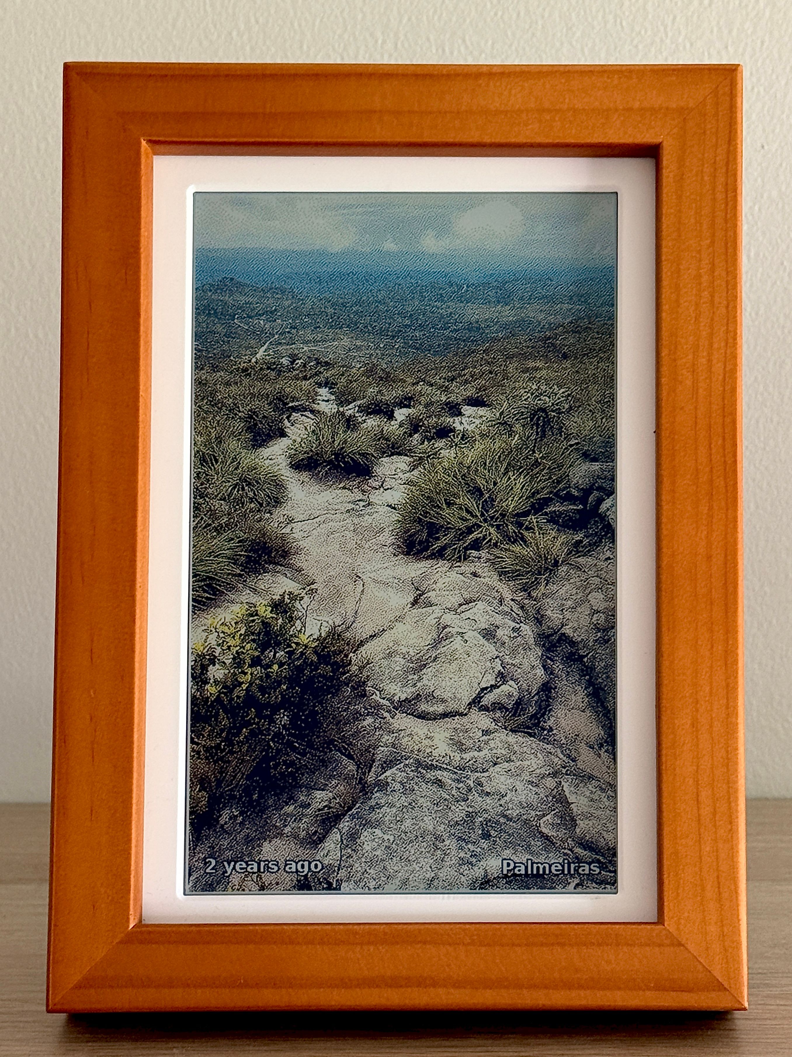
The frame showing a dithered landscape with a small overlay reading '2 years ago' and 'Palmeiras'.

I built a small e-ink photo frame for our home. It pulls photos from a self-hosted Immich1 library, which has already run face detection and geocoding on them. It checks a self-hosted Home Assistant2 instance to see whether anyone is home, then displays a photo on the PhotoPainter3 for everyone to enjoy.

Why

Most digital frames offer a choice between two bad options: preprocess the photos and copy them to an SD card yourself, or hand your library to a cloud service like Google Photos. Realistically, the SD card gets updated once a year, and I’d rather not give a cloud provider access to my most cherished memories.

Yet I’d imagined that coming home to a photo from earlier that day, or one from five years ago, would feel different if it were in a real picture frame instead of buried on my phone. So I decided to spend a weekend building a personal version with Claude Code. I experimented with dithering and post-processing, fine-tuned the photo-picking algorithm, and ended up with this project.

It only took a weekend because so much came for free. Immich had already detected faces in every photo and reverse-geocoded the place names shown on the overlay, and it knew which photos we’d marked as favourites. Home Assistant already knew who everyone was and who was home. That’s the compounding return of self-hosting: every service exposes an easy-to-integrate API, and each new project gets to stand on all of them.

How it works

The frame is driven by a Raspberry Pi Zero 2 W, which is way overpowered, but at least it’s fast enough to let me write plain Python and mostly ignore performance. A cron job runs a script every 15 minutes. Each run:

  1. Quits if it’s between midnight and 7 am. The e-ink display holds its image without power, so the last photo of the evening simply stays up overnight.
  2. Asks Home Assistant whether anyone is home. If not, it quits; there’s no point wasting power and straining the display.
  3. Picks a random photo from Immich, drawn from four overlapping pools: “on this day” memories, favourites, the last 30 days, and the whole library. A rolling 7-day history log prevents repeats. Photos matching the frame’s orientation get 4× the weight, while any candidate whose crop would clip a head is rejected (more on that below).
  4. Crops around any detected faces, boosts contrast and saturation (e-ink is short on both), dithers the image down to the six-colour palette, and pushes the result to the panel. The photo’s age and EXIF location are painted into the bottom corners as white text with a black stroke, so the dither can’t smear the edges.

Image pipeline

The final look depends most on two choices: how the image is cropped around faces and how dithering is applied.

Cropping

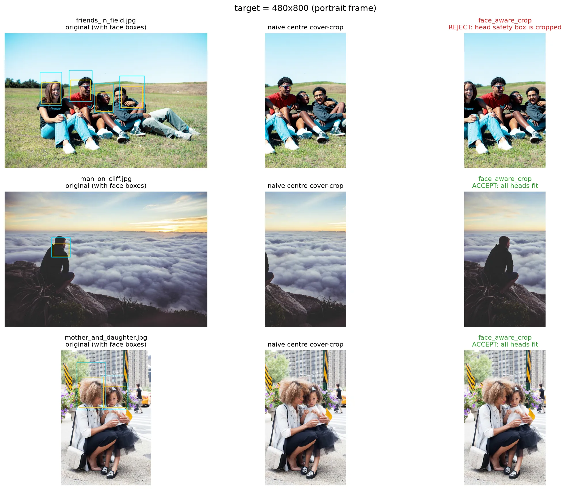
The photo frame stands in one orientation, but I didn’t want to limit it to photos that happen to match. A face-aware algorithm therefore resizes and crops each image to fill the panel, biasing the crop window towards faces Immich has already detected. A landscape shot with some room around the subject will often crop cleanly to portrait this way. If the crop would cut into a head, the photo is rejected and the picker moves to the next candidate.

The examples below show how the head bounding boxes steer the final crop and which candidates get rejected.

Dithering

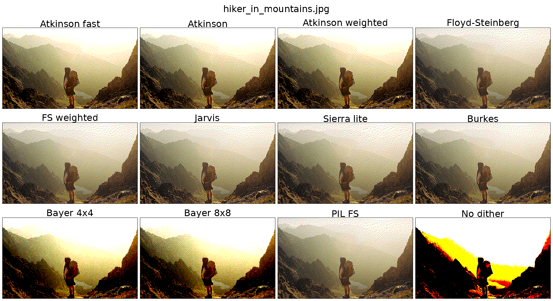
The panel shows exactly six colours: black, white, red, yellow, blue, and green. Unlike an LCD, it has no intensity control, so every pixel must use one of those six colours. Anything photo-like has to be dithered, and the available algorithms differ wildly in output quality and running time. Here’s how a few of them compare:

I settled on Atkinson dithering4, which preserved the most contrast without too many visible artefacts. Unlike the alternatives, it diffuses only 6/8 of each pixel’s quantisation error, so highlights stay bright instead of being dragged grey by their neighbours. Dithering was also the first part of the pipeline where pure Python became unusably slow on the Pi. The inner loop5, including perceptually weighted nearest-colour matching, is therefore JIT-compiled with Numba6. Once the cache is warm, it runs roughly two orders of magnitude faster.

Learnings

The Pi Zero 2 W is overkill. It drains a battery far too quickly: it wastes power sitting idle for most of its life, waiting for the next cron tick. An external RTC-controlled power circuit could have fixed that, but I couldn’t be bothered to hack one in. For a battery-powered build, I’d use an ESP32 with deep sleep instead. With 15 minutes between refreshes, even a slow chip has plenty of time for image processing and dithering.

A few reliability quirks are worth mentioning. In my setup, the Zero 2 W’s Wi-Fi connection drops when power saving kicks in, so a separate cron job runs wifi-check.sh every 5 minutes to reconnect. I also masked swap and set journald to volatile because SD-card wear is the only thing likely to slowly kill the frame.

For the next frame, I’d like to try an Inky Impression7 in a custom enclosure, with a larger display and perhaps integrated lighting. E-ink looks a little muddled in evening light, so a dedicated light source would be the biggest improvement by far.

All in all, the frame already does its job. It stands in the living room as a pleasant speck of curiosity, subtle enough that most visitors never notice it until I inevitably point it out. Once you know it’s there, catching the panel mid-refresh brings a small rush of excitement.

  1. Immich: https://immich.app/
  2. Home Assistant: https://www.home-assistant.io/
  3. PhotoPainter: https://www.waveshare.com/wiki/PhotoPainter
  4. Atkinson dithering: https://en.wikipedia.org/wiki/Atkinson_dithering
  5. inner loop: https://home.schmelczer.dev/git/andras/frame/src/commit/c0c2b779d7b43793b594b9c52b694133859edfd8/src/lib/waveshare_epd/epd7in3e.py#L59-L109
  6. Numba: https://numba.pydata.org/
  7. Inky Impression: https://shop.pimoroni.com/products/inky-impression?variant=55186435244411
Crop comparison showing original photos with face boxes, naive centre crops, and face-aware crops for a portrait frame target, with one candidate rejected for cutting into a head
Palette-preserving dither comparison showing several 6-colour algorithms applied to a hiker in the mountains

Conflict-Free Three-Way Text Merging

Both sides' edits survive without conflict markers, and even the cursors get shifted. Available as a library for Rust, TypeScript, and Python.

The reconcile-text logo and tagline "Conflict-free 3-way text merging".

Why

Merging concurrent edits is a solved problem when you control the whole editing stack1: conflict-free replicated data types2 (CRDTs) and operational transformation3 (OT) capture changes as they happen, which works well when you own the editor, transport layer, and storage format. However, there are workflows where that’s not the case.

For instance, text files on disk can be edited in Obsidian4, Vim, or VS Code and updated through Syncthing or even OneDrive. A sync engine therefore sees only the resulting file snapshots, often after a delay, rather than the individual edits that produced them. This is the same constraint Git works under: Git-tracked files may be edited by many programs, all outside Git’s control. Git rightly highlights ambiguous write-write conflicts with <<<<<<< markers: a bad source-code merge may introduce a bug, so a human should verify the result.5

But I wanted fully automated merges for my text files. That’s why I created reconcile-text, which is built on the assumption that human languages are more forgiving than code: a slightly imperfect sentence is usually better than conflict markers interrupting a document. So reconcile-text essentially implements git merge (technically, it’s git merge-file6) without conflict markers. And it does this without client-side tombstones or an operation history. Let’s look at an example:

import { reconcile } from 'reconcile-text';

// the version both sides start from
const parent = 'Hello world';

// one user added "beautiful"
const left = 'Hello beautiful world';

// the other changed the greeting
const right = 'Hi world';

// "Hi beautiful world"
reconcile(parent, left, right).text;

You can try it out yourself in the interactive playground at reconcile.schmelczer.dev7.

The API is essentially just this one function, plus a few helpers to make transport easier. It takes a parent and two diverging versions, derives and applies both sets of changes, and repositions cursors and selections along the way. Cursor support makes it possible to use reconcile-text in a text editor too.

How it works

The first step is splitting the inputs into tokens, which is why the demo website offers a choice of tokeniser. Even though human text is forgiving of merge artefacts, I still wouldn’t want the characters within words (technically, UTF-8 grapheme clusters) interleaved into nonsense. That’s why treating words, or even sentences, as atoms can be useful. The built-in Markdown tokeniser extends word tokenisation to account for Markdown syntax. The Rust API also lets you specify custom tokenisation rules. We can’t guarantee that the merged Markdown, or other marked-up text, will be syntactically correct8, but we can guarantee that tokens won’t be split up.

After tokenising, the algorithm diffs each edited version against the parent (diff(parent, left), diff(parent, right)), as diff39 does. It uses Myers’ diff algorithm10 to compute those diffs, then cleans them up to make insertions and deletions contiguous, keeping as many of each side’s changes together as possible.

Finally, the two sides are zipped together using OT principles: each side’s edits are transformed against the other side’s. Cursor offsets are updated along the way, making each cursor “stick” to the nearest token and travel with it during the merge.

I didn’t set out to implement OT for its own sake. Transforming batched diffs simply turned out to be an elegant way to merge the outputs of two Myers diffs. A CRDT could achieve the same result. But when all you can observe is the final state, merge quality is limited by the underlying two-way diffs, regardless of the machinery used to combine them.

How to implement a syncer

The library’s merging primitive can support a wide range of text-syncing apps, including ones inspired by differential synchronisation11. A simple starting point is Git’s fetch-merge-push loop, with reconcile-text handling conflicts automatically. An implementation could work as follows:

The server keeps immutable versions of each document, each with a unique ID, and tracks which is the latest. Each client has an editable file and remembers the ID and content hash of the last server version it incorporated. Let’s call that version the base. The client gets it from an initial fetch; after that, it only needs to fetch the base’s text when a merge is necessary.

For each document, the client runs one sync loop at a time:

  1. Check for local edits. Take a snapshot of the file and compare its hash with the base’s hash. If they differ, push the snapshot along with the base’s ID to the server.

  2. Accept if the server hasn’t moved on. The server saves the snapshot only if the base is still its latest version. Checking the ID, saving the new version, and making it the latest happen atomically. Otherwise, it rejects the push and returns its latest version’s ID and text.

  3. On success, remember what was sent. Record the returned ID and the pushed snapshot’s hash as the new base. Keep the live file as it is: the user may have edited it while the request was in flight.

  4. On rejection, merge locally. Fetch the old base’s text and merge it with the current file and the server’s latest text. Record that latest server version’s ID and hash as the new base. The local merge12 is just the same three-way call as before:

    file = reconcile(base, file, latest.text).text;

After either outcome, check for local edits again. A merge may need pushing, and so may edits made during a successful push. The loop pauses once the file’s hash matches the base’s hash, then wakes on local edits, a timer, or a server notification. The timer or notification triggers a fetch: if the server’s version ID has changed, merge and update the base as above, even if the local file hasn’t changed.

Extensions

A real sync app also needs to handle lost responses and application crashes. Giving each push a unique idempotency key lets the client safely retry it: if the server already accepted it, the server can return the original acknowledgement.

To save bandwidth after a merge, the client can use to_diff13 to send only the changes relative to the fetched server version. The server reconstructs the snapshot with from_diff14 and its stored copy of that version.

If fairness becomes an issue, we can let a high-latency client lease a server-side lock long enough to get its edits through.

Where reconcile-text sits among alternatives

diff3 and git merge-file do the hard work of merging but explicitly don’t resolve most write-write conflicts. Neil Fraser’s diff-match-patch is the closest tool in spirit, but it applies two-way patches heuristically rather than reasoning over a common ancestor and both edited versions. So failed patches can lose edits. CRDTs preserve concurrent edits, but they require CRDT state and metadata tied to the document’s editing history rather than three plain strings. That’s the niche reconcile-text fills: syncing systems that need automatic merges but only have snapshots to work with.

One implementation, many ecosystems

The Rust library compiles to WebAssembly through wasm-bindgen15 for the npm package and provides native Python bindings through PyO316. This makes reconcile-text available from Rust, Python, and JavaScript or TypeScript across Node.js, the web, and React Native. Since React Native’s Hermes engine doesn’t support WebAssembly, that entry point ships a pure-JavaScript build produced by Binaryen’s wasm2js.

  1. a solved problem when you control the whole editing stack: https://marijnhaverbeke.nl/blog/collaborative-editing-cm.html
  2. conflict-free replicated data types: https://crdt.tech/
  3. operational transformation: https://en.wikipedia.org/wiki/Operational_transformation
  4. Obsidian: https://obsidian.md/
  5. Semantic merge conflicts can still slip past Git without producing conflict markers.
  6. git merge-file: https://git-scm.com/docs/git-merge-file
  7. https://reconcile.schmelczer.dev/
  8. Ink & Switch’s Peritext17 is a good write-up on this problem for rich text.
  9. diff3: https://blog.jcoglan.com/2017/05/08/merging-with-diff3/
  10. Myers’ diff algorithm: https://blog.jcoglan.com/2017/02/12/the-myers-diff-algorithm-part-1/
  11. differential synchronisation: https://neil.fraser.name/writing/sync/
  12. local merge: https://home.schmelczer.dev/git/andras/reconcile/src/commit/08a656c6ed32d7c307b36bc6dec0134c40ac0a43/reconcile-js/src/core.ts
  13. to_diff: https://home.schmelczer.dev/git/andras/reconcile/src/commit/08a656c6ed32d7c307b36bc6dec0134c40ac0a43/src/operation_transformation/edited_text.rs#L406
  14. from_diff: https://home.schmelczer.dev/git/andras/reconcile/src/commit/08a656c6ed32d7c307b36bc6dec0134c40ac0a43/src/operation_transformation/edited_text.rs#L475
  15. wasm-bindgen: https://docs.rs/wasm-bindgen
  16. PyO3: https://pyo3.rs/
  17. Peritext: https://www.inkandswitch.com/peritext

Turning Linear Search into a Performant Data Processing Engine

Filter 25 million property records by 87 criteria in under 100 ms (p99) to help decide where to buy a home.

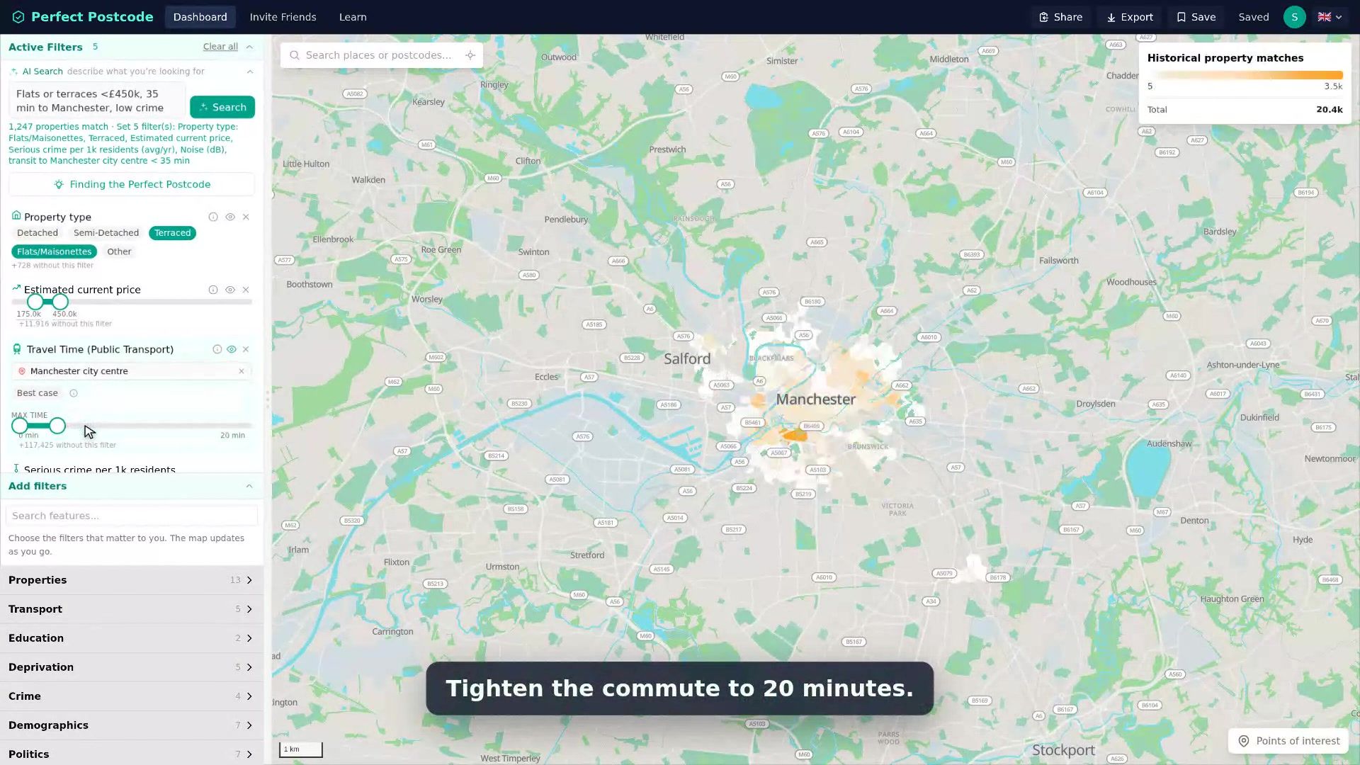
The Perfect Postcode dashboard with active filters on property type, price, transit time, and crime, showing a Manchester map with matching properties highlighted as a heatmap.

The pitch

There’s an immense amount of public, highly granular data about the UK, especially England and Wales: the price of every property transaction1; floor areas and construction years2, all with full addresses; street-level crime3; noise levels at 10 m by 10 m granularity4; public transport timetables5; mapped woodlands6; conservation areas, council houses, listed buildings7, and schools8; plus detailed demographics9 on education, renting, and a lot more. When I was looking to buy a property, these datasets helped me narrow down where to move and what to expect.

Sites such as HouseMetric10 and CrystalRoof11 already provide some of this data for a given postcode, but I needed the search the other way around. I had been living in London for only four years, so I didn’t know its many neighbourhoods well enough. That’s why I wanted to flip the lookup: instead of going from a postcode to its attributes, I wanted to go from the description of my ideal area to matching postcodes. This is how perfect-postcode.co.uk12 began.

Perfect Postcode introduced me to several hidden gems I’d never heard of but fell in love with after visiting. It pushed me beyond familiar areas and gave me a broader picture of London. It also showed me what my expectations would cost and how the equation changed with a compromise or two.

In short, users can set minimum and maximum values for each property and area attribute. For example, a user can ask to see only areas within a 10-minute walk of a station, with noise below 56 dB, with a 2-bed costing less than £600k, plus any of the 83 other criteria. The result is a heatmap showing which areas contain the highest number of matching past sales, and therefore where the criteria are most likely to be met. From there, users can narrow their search, contact estate agents, get access to off-market properties, and keep an eye on Rightmove and Zoopla.

Rough architecture

Filtering happens per property: all the public data is joined onto roughly 25 million property records which are than aggregated at various granularities. Matches appear as H313 hexagons at lower zoom levels and postcode boundaries at the highest zoom.

The basic architecture is straightforward: download the data, normalise and join it, add a filtering UI, then write a backend that returns matching areas. The difficult part is the main non-functional requirement: filtering must feel instant so users can see how each change affects the results to allow developing an intuition.

The full dataset contains 25 million rows. That’s really not that much data for today’s servers; it’s not too large to keep in memory, and it also won’t grow exponentially. That’s why I decided to see how far a brute-force linear scan could take me with it. Making brute force fast requires some preparation. So most attributes are quantised to 16 bits because values such as crime counts and room counts need no greater range or precision. There is only one index: a spatial grid (0.01 deg) that prunes addresses outside the user’s viewport. The data uses a row-major layout because queries often filter on dozens of attributes at once. Rows are also sorted by spatial position, so each scan touches contiguous chunks. This keeps scans cache-friendly and easy to parallelise.

After the intentional data layout, the brute-force search logic is as simple as for each row:

let base = row * NUM_FEATURES;
let should_include = filters.iter().all(|f| {
    let raw = feature_data[base + f.feat_idx];
    raw != NAN_U16 && raw >= f.min_u16 && raw <= f.max_u16
})

In practice, this results in sub-100 ms p99 query latency for our userbase which easily justifies the server’s roughly 12 GB memory footprint.

Still, 100 ms plus network latency is too slow for instantaneous feedback in the UI. Fortunately, filters are always combined with AND, and users can adjust only one at a time by changing that attribute’s bounds. This allows a simple trick: when a user starts adjusting a filter, the frontend requests that attribute’s minimum and maximum values for every visible hexagon or postcode. It can then update the colours and filtering without another round trip by applying a single attribute’s filter client-side. You can see both the backend and frontend optimisations in action together here:

Of course, there’s a bit more to it, especially at the coarser H3 levels, where expensive queries benefit most from caching. Other data stays outside the hot path, including individual property histories and travel times. But the short version is that brute force can be the best solution when applied in a smart way.

Derived data

Besides the open datasets, the pipelines powering the app create interesting derived values, for example:

  • Tree canopy density percentile: based on mapped tree-canopy and woodland coverage
  • Price growth percentile: showing where prices are rising or falling fastest
  • Public transport travel time: calculated between stations and neighbourhoods using R514 which is precomputed for every postcode and destination combination under several constraints

What’s next?

Six months of viewings and scouting areas in-person gave the perfect feedback loop. Whenever the numbers and my impression of an area differed, it usually pointed to a missing feature. For example, one Saturday we visited an area of Loughton that had looked perfect based on the numbers. However, we counted more than a dozen England flags hanging from properties, which prompted me to add a Reform UK voter share filter. Now that the product works well for us, it’s time to iterate on user feedback.

Originally, the app’s target audience was my fiancée and I. But as we added features, it became clear that other house hunters could benefit from it too. That meant improving the user experience with saved and shareable filters, clearer explanations, and a genuinely usable mobile site, then adding a payment flow and doing some marketing. Now, we’re looking at the usage metrics to see where to take the project from here.

  1. price of every property transaction: https://www.gov.uk/guidance/about-the-price-paid-data
  2. floor areas and construction years: https://epc.opendatacommunities.org/
  3. street-level crime: https://data.police.uk/
  4. noise levels at 10 m by 10 m granularity: https://environment.data.gov.uk/dataset/562c9d56-7c2d-4d42-83bb-578d6e97a517
  5. public transport timetables: https://www.bus-data.dft.gov.uk/
  6. woodlands: https://www.forestresearch.gov.uk/tools-and-resources/national-forest-inventory/
  7. listed buildings: https://opendata-historicengland.hub.arcgis.com/
  8. schools: https://get-information-schools.service.gov.uk/
  9. detailed demographics: https://www.ons.gov.uk/census
  10. HouseMetric: https://housemetric.co.uk/
  11. CrystalRoof: https://crystalroof.co.uk/
  12. https://perfect-postcode.co.uk/
  13. H3: https://h3geo.org/
  14. R5: https://conveyal.com/

Searches titles, descriptions, and the full text of every article.

    to move to open Esc to close